Linear Multistep Methods
Author:
Philip Osborne
Last Updated:
12 лет назад
License:
Creative Commons CC BY 4.0
Аннотация:
Part 3 project plan

\begin
Discover why over 25 million people worldwide trust Overleaf with their work.

\begin
Discover why over 25 million people worldwide trust Overleaf with their work.
\documentclass[11pt]{article}

\usepackage[sort]{natbib}
\usepackage{fancyhdr}

% you may include other packages here (next line)
\usepackage{enumitem}


%----- you must not change this -----------------
\oddsidemargin 0.2cm
\topmargin -1.0cm
\textheight 24.0cm
\textwidth 15.25cm
\parindent=0pt
\parskip 1ex
\renewcommand{\baselinestretch}{1.1}
\pagestyle{fancy}
%----------------------------------------------------


% enter your details here----------------------------------

\lhead{\normalsize \textrm{Part 3 Project (Project Plan)}}
\chead{}
\rhead{\normalsize 21015604}
\lfoot{\normalsize \textrm{MA3PR}}
\cfoot{}
\rfoot{Dr Polly J. Smith}
\setlength{\fboxrule}{4pt}\setlength{\fboxsep}{2ex}
\renewcommand{\headrulewidth}{0.4pt}
\renewcommand{\footrulewidth}{0.4pt}


\begin{document}


%----------------your title below -----------------------------

\begin{center}
{\bf Linear Multistep methods }
\end{center}


%---------------- start of document body------------------
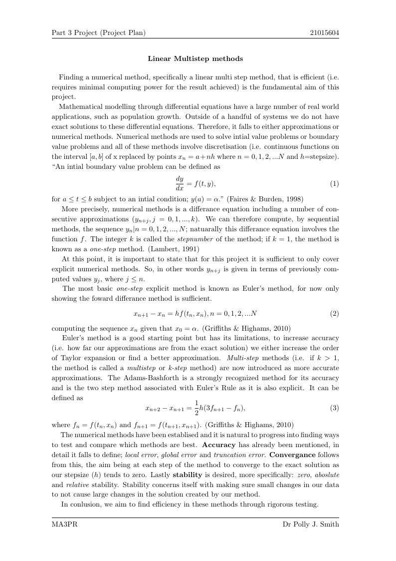
\hspace*{1em}Finding a numerical method, specifically a linear multi step method, that is efficient (i.e. requires minimal computing power for the result achieved) is the fundamental aim of this project.\\
\hspace*{1em}Mathematical modelling through differential equations have a large number of real world applications, such as population growth. Outside of a handful of systems we do not have exact solutions to these differential equations. Therefore, it falls to either approximations or numerical methods. Numerical methods are used to solve intial value problems or boundary value problems and all of these methods involve discretisation (i.e. continuous functions on the interval $[a,b]$ of x replaced by points $x_{n}=a+nh$ where $n=0,1,2,...N$ and $h$=stepsize).\\
``An intial boundary value problem can be defined as
\begin{equation}
\frac{dy}{dx}=f(t,y),
\end{equation}
for $a\leq t\leq b$ subject to an intial condition; $y(a)=\alpha$."  \citep{Faires}\\
\hspace*{1em}    More precisely, numerical methods is a differance equation including a number of consecutive approximations ($y_{n+j},j=0,1,...,k$). We can therefore compute, by sequential methods, the sequence {$y_{n}|n=0,1,2,...,N$}; natuarally this differance equation involves the function $f$. The integer $k$ is called the \textit{stepnumber} of the method; if $k=1$, the method is known as a \textit{one-step} method. \citep{Lambert1991}\\
\hspace*{1em}    At this point, it is important to state that for this project it is sufficient to only cover explicit numerical methods. So, in other words $y_{n+j}$ is given in terms of previously computed values $y_{j}$, where $j\leq n$.\\
\hspace*{1em}    The most basic \textit{one-step} explicit method is known as Euler's method, for now only showing the foward differance method is sufficient.
\begin{equation}
x_{n+1}-x_{n} = hf(t_{n},x_{n}), n=0,1,2,...N
\end{equation}
computing the sequence {$x_{n}$} given that $x_{0}=\alpha$. \citep{Griffiths}\\
\hspace*{1em}    Euler's method is a good starting point but has its limitations, to increase accuracy (i.e. how far our approximations are from the exact solution) we either increase the order of Taylor expansion or find a better approximation. \textit{Multi-step} methods (i.e. if $k>1$, the method is called a \textit{multistep} or \textit{k-step} method)
are now introduced as more accurate approximations. The Adams-Bashforth is a strongly recognized method for its accuracy and is the two step method associated with Euler's Rule as it is also explicit. It can be defined as
\begin{equation}
x_{n+2}-x_{n+1}=\frac{1}{2}h(3f_{n+1}-f_{n}),
\end{equation}

where $f_{n}=f(t_{n},x_{n})$ and $f_{n+1}=f(t_{n+1},x_{n+1})$. \citep{Griffiths}\\
\hspace*{1em}   The numerical methods have been establised and it is natural to progress into finding ways to test and compare which methods are best. \textbf{Accuracy} has already been mentioned, in detail it falls to define; \textit{local error}, \textit{global error} and \textit{truncation error}. \textbf{Convergance} follows from this, the aim being at each step of the method to converge to the exact solution as our stepsize ($h$) tends to zero. Lastly \textbf{stability} is desired, more specifically: \textit{zero}, \textit{aboslute} and \textit{relative} stability. Stability concerns itself with making sure small changes in our data to not cause large changes in the solution created by our method.\\
\hspace*{1em}    In conlusion, we aim to find efficiency in these methods through rigorous testing.


% ----------------end of document body---------------------

%---------------- start of references------------------

\begin{thebibliography}{999}
\bibitem[Faires \& Burden(1998)]{Faires}{Faires.D.J \& Burden.R. (1998). \textit{Numerical methods: second edition}. USA: Brooks/Cole Publishing Company}
\bibitem[Griffiths \& Highams(2010)]{Griffiths}{Griffiths.D.F. \& Highams.D.J.(2010). \textit{Numerical methods for Ordinary Differential equations: Initial Value Problems}. London: Springer Undergraduate Mathematics series.}
% ---Not currently cited but kept in for future referance----\bibitem[Lambert(1973)]{Lambert1973}{Lambert.J.D.(1973). \textit{Computation Methods in Ordinary Differential Equations}, New York: John Wiley \& Sons.}
\bibitem[Lambert(1991)]{Lambert1991}{Lambert.J.D.(1991). \textit{Numerical Methods for Ordinary Differential Systems: The Initial Value Problem}, West Sussex: John Wiley \& Sons Ltd.}


\end{thebibliography}

%---------------- end of references------------------


\end{document}